Patozone

Vectors

 

Creating and naming Vectors
Vectors are sequences of data elements c same basic type

- can be characters, numeric or logical

 

Creating vectors c(); naming vectors names()

> remain <- c(11, 12, 11, 13)

> remain

[1] 11 12 11 13

> suits <- c("spades", "hearts", "diamonds", "clubs")

> names(remain) <- suits

> remain

spades hearts diamonds clubs

11 12 11 13

 

> remain <- c(spades = 11, hearts = 12,

diamonds = 11, clubs = 13)

 

> remain <- c("spades" = 11, "hearts" = 12,

"diamonds" = 11, "clubs" = 13)

 

Option 1

> remain <- c(11, 12, 11, 13)

> suits <- c("spades", "hearts", "diamonds", "clubs")

> names(remain) <- suits

 

Option 2

> remain <- c(spades = 11, hearts = 12,

diamonds = 11, clubs = 13)

 

Option 3

> remain <- c("spades" = 11, "hearts" = 12,

"diamonds" = 11, "clubs" = 13)

 

> str(remain)

Named num [1:4] 11 12 11 13

- attr(*, "names")= chr [1:4] "spades" "hearts"

"diamonds" "clubs"

 

Single value = vector

> my_apples <- 5

> my_oranges <- "six"

 

> is.vector(my_apples)

[1] TRUE

> is.vector(my_oranges)

[1] TRUE

 

> length(my_apples)

[1] 1

> length(my_oranges)

[1] 1

> length(drawn_suits)

[1] 5

 

Vectors are homogeneous

Only elements of the same type; atomic vectors < > lists

- auto coercion if necessary

 

> drawn_ranks <- c(7, 4, "A", 10, "K", 3, 2, "Q")

> drawn_ranks

[1] "7" "4" "A" "10" "K" "3" "2" "Q"

> class(drawn_ranks)

[1] "character"

 

Vector Arithmetic

> my_apples <- 5

> my_oranges <- 6

> my_apples + my_oranges

[1] 11

 

Computations are performed element-wise

> earnings <- c(50, 100, 30)

> earnings * 3

[1] 150 300 90

 

#Mathematics naturally extended

> earnings/10

[1] 5 10 3

> earnings - 20

[1] 30 80 10

> earnings + 100

[1] 150 200 130

> earnings^2

[1] 2500 10000 900

 

Element-wise

> earnings <- c(50, 100, 30)

> expenses <- c(30, 40, 80)

> earnings - expenses

[1] 20 60 -50

> earnings + c(10, 20, 30)

[1] 60 120 60

> earnings * c(1, 2, 3)

[1] 50 200 90

> earnings / c(1, 2, 3)

[1] 50 50 10

 

sum() and >

> earnings <- c(50, 100, 30)

> expenses <- c(30, 40, 80)

> bank <- earnings - expenses

> bank

[1] 20 60 -50

> sum(bank)

[1] 30

> earnings > expenses

[1] TRUE TRUE FALSE

Subsetting Vectors

Subset by index

> remain <- c(spades = 11, hearts = 12,

diamonds = 11, clubs = 13)

> remain[1]       [1] -> take element at index 1

spades              result is spades a (named) vector too!

11

> remain[3]

diamonds

11

 

Subset by name

> remain <- c(spades = 11, hearts = 12,

diamonds = 11, clubs = 13)

> remain["spades"]

spades

11

> remain["diamonds"]

diamonds

11

 

Subset multiple elements

> remain <- c(spades = 11, hearts = 12,

diamonds = 11, clubs = 13)

> remain_black <- remain[c(1, 4)]

> remain_black

spades clubs

11 13

> remain[c(4, 1)]     #order in selection vector matters!

clubs spades

13       11

> remain[c("clubs", "spades")]

clubs spades

13 11

 

Subset all but some

> remain <- c(spades = 11, hearts = 12,

diamonds = 11, clubs = 13)

> remain[-c(1, 2)]

diamonds clubs

11              13

> remain[-"spades"]

Error in -"spades" : invalid argument to unary operator

hearts diamonds clubs All but index 1 are returned

12 11 13

> remain[-1]

 

Subset using logical vector

> remain <- c(spades = 11, hearts = 12,

diamonds = 11, clubs = 13)

> remain[c(FALSE, TRUE, FALSE, TRUE)]

hearts clubs

12         13

> selection_vector <- c(FALSE, TRUE, FALSE, TRUE)

> remain[selection_vector]

hearts clubs

12 13

 

Subset using logical vector

> remain <- c(spades = 11, hearts = 12,

diamonds = 11, clubs = 13)

> remain[c(TRUE, FALSE)]     #Recycles to c(T,F,T,F)

spades diamonds

11 11

> remain[c(TRUE, FALSE, TRUE, FALSE)]

spades diamonds

11 11

> remain[c(TRUE, FALSE, TRUE)]

spades diamonds clubs

11 11 13

> remain[c(TRUE, FALSE, TRUE, TRUE)]

spades diamonds clubs

11 11 13

Matrices

 

Creating and Naming Matrices

● Vector: 1D array of data elements

● Matrix: 2D array of data elements

● Rows and columns

● One atomic vector type

 

Create a matrix: matrix()

> matrix(1:6, nrow = 2)

[,1] [,2] [,3]

[1,] 1 3 5

[2,] 2 4 6

> matrix(1:6, ncol = 3)

[,1] [,2] [,3]

[1,] 1 3 5

[2,] 2 4 6

> matrix(1:6, nrow = 2, byrow = TRUE)

[,1] [,2] [,3]

[1,] 1 2 3

[2,] 4 5 6

 

Create a matrix: recycling

> matrix(1:3, nrow = 2, ncol = 3)

[,1] [,2] [,3]

[1,] 1 3 2

[2,] 2 1 3

> matrix(1:4, nrow = 2, ncol = 3)

[,1] [,2] [,3]

[1,] 1 3 1

[2,] 2 4 2

Warning message:

In matrix(1:4, nrow = 2, ncol = 3) :

data length [4] is not a sub-multiple or multiple of the

number of columns [3]

 

rbind() and cbind()

> cbind(1:3, 1:3)

[,1] [,2]

[1,] 1 1

[2,] 2 2

[3,] 3 3

> rbind(1:3, 1:3)

[,1] [,2] [,3]

[1,] 1 2 3

[2,] 1 2 3

 

> m <- matrix(1:6, byrow = TRUE, nrow = 2)

> rbind(m, 7:9)

[,1] [,2] [,3]

[1,] 1 2 3

[2,] 4 5 6

[3,] 7 8 9

> cbind(m, c(10, 11))

[,1] [,2] [,3] [,4]

[1,] 1 2 3 10

[2,] 4 5 6 11

 

Naming a matrix with rownames() and colnames()

> m <- matrix(1:6, byrow = TRUE, nrow = 2)

> rownames(m) <- c("row1", "row2")

[,1] [,2] [,3]

row1 1 2 3

row2 4 5 6

> m

> colnames(m) <- c("col1", "col2", "col3")

> m

col1 col2 col3

row1 1 2 3

row2 4 5 6

 

Naming a matrix

> m <- matrix(1:6, byrow = TRUE, nrow = 2,

dimnames = list(c("row1", "row2"),

c("col1", "col2", "col3")))

> m

col1 col2 col3

row1 1 2 3

row2 4 5 6

 

Coercion

> num <- matrix(1:8, ncol = 2)

> num

[,1] [,2]

[1,] 1 5

[2,] 2 6

[3,] 3 7

[4,] 4 8

> char <- matrix(LETTERS[1:6], nrow = 4, ncol = 3)

> char

[,1] [,2] [,3]

[1,] "A" "E" "C"

[2,] "B" "F" "D"

[3,] "C" "A" "E"

[4,] "D" "B" "F"

 

> num <- matrix(1:8, ncol = 2)

> char <- matrix(LETTERS[1:6], nrow = 4, ncol = 3)

> cbind(num, char)

[,1] [,2] [,3] [,4] [,5]

[1,] "1" "5" "A" "E" "C"

[2,] "2" "6" "B" "F" "D"

[3,] "3" "7" "C" "A" "E"

[4,] "4" "8" "D" "B" "F"

 

If it contains different types, list or data.frame

 

Matrix Subsetting

 

Subset element

> m <- matrix(sample(1:15, 12), nrow = 3)

> m

[,1] [,2] [,3] [,4]

[1,] 5 11 15 3

[2,] 12 14 8 9

[3,] 6 1 4 2

> m[1,3]

[1] 15

> m[3,2]

[1] 1

 

Subset column or row

> m

[,1] [,2] [,3] [,4]

[1,] 5 11 15 3

[2,] 12 14 8 9

[3,] 6 1 4 2

 

> m[3,]

[1] 6 1 4 2

> m[,3]

[1] 15 8 4

> m[4]

[1] 11

> m[9]

[1] 4

 

Subset multiple elements

> m

[,1] [,2] [,3] [,4]

[1,] 5 11 15 3

[2,] 12 14 8 9

[3,] 6 1 4 2

 

> m[2, c(2, 3)]

[1] 14 8

> m[c(1, 2), c(2, 3)]

> m[c(1, 3), c(1, 3, 4)]

[,1] [,2]

[1,] 11 15

[2,] 14 8

[,1] [,2] [,3]

[1,] 5 15 3

[2,] 6 4 2

 

Subset by name

> rownames(m) <- c("r1", "r2", "r3")

> colnames(m) <- c("a", "b", "c", "d")

> m

    a  b   c  d

r1 5 11 15 3

r2 12 14 8 9

r3 6 1 4 2

> m[2,3]

[1] 8

> m["r2","c"]

[1] 8

> m[2,"c"]

[1] 8

> m[3, c("c", "d")]

c d

4 2

 

Subset with logical vector

> m

a b c d

r1 5 11 15 3

r2 12 14 8 9

r3 6 1 4 2

 

> m[c(FALSE, FALSE, TRUE),

c(FALSE, FALSE, TRUE, TRUE)]

c d

4 2

> m[c(FALSE, FALSE, TRUE),

c(FALSE, TRUE)]

b d

1 2

> m[c(FALSE, FALSE, TRUE),

c(FALSE, TRUE, FALSE, TRUE)]

b d

1 2

 

Matrix Arithmetic

 

● colSums(), rowSums()

● Standard arithmetic possible

● Element-wise computation

 

lotr_matrix

> the_fellowship <- c(316, 556)

> two_towers <- c(343, 584)

> return_king <- c(378, 742)

> lotr_matrix <- rbind(the_fellowship, two_towers, return_king)

> colnames(lotr_matrix) <- c("US", "non-US")

> rownames(lotr_matrix) <- c("Fellowship", "Two Towers",

"Return King")

> lotr_matrix

US non-US

Fellowship 316 556

Two Towers 343 584

Return King 378 742

 

Matrix Scalar

> lotr_matrix

US non-US

Fellowship 316 556

Two Towers 343 584

Return King 378 742

 

> lotr_matrix / 1.12

US non-US

Fellowship 282.1429 496.4286

Two Towers 306.2500 521.4286

Return King 337.5000 662.5000

> lotr_matrix - 50

US non-US

Fellowship 266 506

Two Towers 293 534

Return King 328 692

 

Matrix - Matrix

> # Definition of theater_cut omitted

> theater_cut

[,1] [,2]

[1,] 50 50

[2,] 80 80

[3,] 100 100

> lotr_matrix - theater_cut

US non-US

Fellowship 266 506

Two Towers 263 504

Return King 278 642

 

Recycling

> lotr_matrix - c(50, 80, 100)

US non-US

Fellowship 266 506

Two Towers 263 504

Return King 278 642

> matrix(c(50, 80, 100), nrow = 3, ncol = 2)

[,1] [,2]

[1,] 50 50

[2,] 80 80

[3,] 100 100

 

Matrix Multiplication

> # Definition of rates omitted

> rates

[,1] [,2]

[1,] 1.11 1.11

[2,] 0.99 0.99

[3,] 0.82 0.82

> lotr_matrix * rates

US non-US

Fellowship 350.76 617.16

Two Towers 339.57 578.16

Return King 309.96 608.44

 

Matrices and Vectors

● Very similar

● Vector = 1D, matrix = 2D

● Coercion if necessary

● Recycling if necessary

● Element-wise calculations

Factors

 

Categorical Variables

● Limited number of different values

● Belong to category

● In R: factor

 

Create a factor: factor()

> blood <- c("B", "AB", "O", "A", "O", "O", "A", "B")

> blood

[1] "B" "AB" "O" "A" "O" "O" "A" "B"

factor()

> blood_factor <- factor(blood)

> blood_factor

[1] B AB O A O O A B   #sorts alphabetically

Levels: A AB B O

> str(blood_factor)

Factor w/ 4 levels "A","AB","B","O": 3 2 4 1 4 4 1 3

 

Order levels differently

> blood_factor2 <- factor(blood,

levels = c("O", "A", "B", "AB"))

> blood_factor2

[1] B AB O A O O A B

Levels: O A B AB

> str(blood_factor2)

Factor w/ 4 levels "O","A","B","AB": 3 4 1 2 1 1 2 3

> str(blood_factor)

Factor w/ 4 levels "A","AB","B","O": 3 2 4 1 4 4 1 3

 

Rename factor levels

> blood <- c("B", "AB", "O", "A", "O", "O", "A", "B")

> blood_factor <- factor(blood)

> levels(blood_factor) <- c("BT_A", "BT_AB", "BT_B", "BT_O")

> blood_factor

[1] BT_B BT_AB BT_O BT_A BT_O BT_O BT_A BT_B

Levels: BT_A BT_AB BT_B BT_O

> factor(blood, labels = c("BT_A", "BT_AB", "BT_B", "BT_O"))

[1] BT_B BT_AB BT_O BT_A BT_O BT_O BT_A BT_B

Levels: BT_A BT_AB BT_B BT_O

 

> blood <- c("B", "AB", "O", "A", "O", "O", "A", "B")

> blood_factor <- factor(blood)

> factor(blood,

levels = c("O", "A", "B", "AB"),

labels = c("BT_O", "BT_A", "BT_B", "BT_AB"))

[1] BT_B BT_AB BT_O BT_A BT_O BT_O BT_A BT_B

Levels: BT_O BT_A BT_B BT_AB

 

Nominal vs Ordinal

> blood <- c("B", "AB", "O", "A", "O", "O", "A", "B")

> blood_factor <- factor(blood)

> blood_factor[1] < blood_factor[2]

[1] NA

Warning message:

In Ops.factor(blood_factor[1], blood_factor[2]) :

‘<’ not meaningful for factors

> tshirt <- c("M", "L", "S", "S", "L", "M", "L", "M")

> tshirt_factor <- factor(tshirt, ordered = TRUE,

levels = c("S", "M", "L"))

> tshirt_factor

[1] M L S S L M L M

Levels: S < M < L

 

Ordered factor

> tshirt <- c("M", "L", "S", "S", "L", "M", "L", "M")

> tshirt_factor <- factor(tshirt, ordered = TRUE,

levels = c("S", "M", "L"))

> tshirt_factor

[1] M L S S L M L M

Levels: S < M < L

> tshirt_factor[1] < tshirt_factor[2]

[1] TRUE

 

Wrap up

● Factors for categorical variables

● Factors are integer vectors

● Change factor levels:

levels() function or labels argument

● Ordered factors: ordered = TRUE

 

 

Factors Lab

 

# Definition of hand_vector

hand_vector <- c("Right", "Left", "Left", "Right", "Left")

 

# Convert hand_vector to a factor: hand_factor

hand_factor <- factor(hand_vector)

 

# Display the structure of hand_factor

str(hand_factor)

 

# Encode survey_vector as a factor with the correct names: survey_factor

survey_factor <- factor(survey_vector, levels = c("L", "R"), labels = c("Left", "Right"))

 

# Print survey_factor

survey_factor

 

# Summarize survey_vector

summary(survey_vector)

 

# Summarize survey_factor

summary(survey_factor)

 

Animals and Temperature

# Definition of animal_vector and temperature_vector

animal_vector <- c("Elephant", "Giraffe", "Donkey", "Horse")

temperature_vector <- c("High", "Low", "High", "Low", "Medium")

 

# Convert animal_vector to a factor: animal_factor

animal_factor <- factor(animal_vector)

 

# Encode temperature_vector as a factor: temperature_factor

temperature_factor <- factor(temperature_vector, ordered = TRUE, levels = c("Low", "Medium", "High"))

 

# Print out animal_factor and temperature_factor

animal_factor

temperature_factor

 

Speed of Data Analysts

# Convert speed_vector to ordered speed_factor

speed_factor <- factor(speed_vector, ordered = TRUE, levels = c("Slow", "OK", "Fast"))

 

# Print speed_factor

speed_factor

 

# Summarize speed_factor

summary(speed_factor)

 

 

# Definition of speed_vector and speed_factor

speed_vector <- c("Fast", "Slow", "Slow", "Fast", "Ultra-fast")

factor_speed_vector <- factor(speed_vector, ordered = TRUE, levels = c("Slow", "Fast", "Ultra-fast"))

 

# Compare DA2 with DA5: compare_them

compare_them <- speed_vector[2] > speed_vector[5]

 

# Print compare_them: Is DA2 faster than DA5?

compare_them

 

 

Lists

 

Creating Names and Lists

● Vector: 1D, same type

● Matrix: 2D, same type

● List

● Different R objects

● No coercion

● Loss of some functionality

 

Create list: list()

> c("Rsome times", 190, 5)

[1] "Rsome times" "190" "5"

 

> list("Rsome times", 190, 5)

[[1]]

[1] "Rsome times"

 

[[2]]

[1] 190

 

[[3]]

[1] 5

 

> song <- list("Rsome times", 190, 5)

> is.list(song)

[1] TRUE

 

Name list

> song <- list("Rsome times", 190, 5)

> names(song) <- c("title", "duration", "track")

 

> song

$title

[1] "Rsome times"

 

$duration

[1] 190

 

$track

[1] 5

 

> song <- list(title = "Rsome times",

duration = 190, track = 5)

 

> str(song)

List of 3

$ title : chr "Rsome times"

$ duration: num 190

$ track : num 5

 

List in List

> similar_song <- list(title = "R you on time?",

duration = 230)

 

> song <- list(title = "Rsome times",

duration = 190, track = 5, similar = similar_song)

 

> str(song)

List of 4

$ title : chr "Rsome times"

$ duration: num 190

$ track : num 5

$ similar :List of 2

..$ title : chr "R you on time?"

..$ duration: num 230

 

Subset and Extend Lists

 

The song list

> similar_song <- list(title = "R you on time?",

duration = 230)

> song <- list(title = "Rsome times",

duration = 190, track = 5,

similar = similar_song)

 

> song

List of 4

$ title : chr "Rsome times"

$ duration: num 190

$ track : num 5

$ similar :List of 2

..$ title : chr "R you on time?"

..$ duration: num 230

 

[ versus [[

> song

List of 4

$ title : chr "Rsome times"

$ duration: num 190

$ track : num 5

$ similar :List of 2

..$ title : chr "R you on time?"

..$ duration: num 230

 

> song[1]

List of 1

   $ title: chr "Rsome times"

 

> song[[1]]

[1] "Rsome times"

 

> song[c(1, 3)]

List of 2

  $ title: chr "Rsome times"

  $ track: num 5

 

> song[[c(1, 3)]]

Error in song[[c(1, 3)]] :

subscript out of bounds

 

> song[[1]][[3]]

Error in song[[1]][[3]] :

subscript out of bounds

 

> song[[4]][[1]]

[1] "R you on time?"

 

> song[[c(4, 1)]]

[1] "R you on time?"

 

Subset by names

> song[["duration"]]

[1] 190

 

> song["duration"]

List of 1

$ duration: num 190

 

> song[c("duration", "similar")]

List of 2

$ duration: num 190

$ similar :List of 2

..$ title : chr "R you on time?"

..$ duration: num 230

 

Subset by logicals

> song[c(FALSE, TRUE, TRUE, FALSE)]

List of 2

$ duration: num 190

$ track : num 5

 

> song[[c(FALSE, TRUE, TRUE, FALSE)]]

Error : attempt to select less than one element

 

> song[[F]][[T]][[T]][[F]]

Error : attempt to select less than one element

 

$ and extending

> song$duration

[1] 190

 

> friends <- c("Kurt", "Florence", "Patti", "Dave")

> song$sent <- friends

> song

List of 5

$ title : chr "Rsome times"

$ duration: num 190

$ track : num 5

$ similar :List of 2

..$ title : chr "R you on time?"

..$ duration: num 230

$ sent : chr [1:4] "Kurt" "Florence" "Patti" "Dave"

 

Extending lists

> song[["sent"]] <- friends

 

> song$similar$reason <- "too long"

 

> song

List of 5

$ title : chr "Rsome times"

$ duration: num 190

$ track : num 5

$ similar :List of 3

..$ title : chr "R you on time?"

..$ duration: num 230

..$ reason : chr "too long"

$ sent : chr [1:4] "Kurt" "Florence" "Patti" "Dave"

 

Wrap up

● [[ or [ ?

● [[ to select list element

● [ results in sublist

● [[ and $ to subset and extend lists

Data Frames

 

Exploring the Data Frame

 

Datasets...

● Observations

● Variables

● Example: people

● each person = observation

● properties (name, age …) = variables

● Matrix?   Need different types

● List?   Not very practical

 

Data Frame!

● Specifically for datasets

● Rows = observations (persons)

● Columns = variables (age, name, …)

● Contain elements of different types

● Elements in same column: same type

 

Creating a Data Frame

● Import from data source

● CSV file

● Relational Database (e.g. SQL)

● Software packages (Excel, SPSS …)

 

Creating a Data Frame: data.frame()

> name <- c("Anne", "Pete", "Frank", "Julia", "Cath")

> age <- c(28, 30, 21, 39, 35)

> child <- c(FALSE, TRUE, TRUE, FALSE, TRUE)

> df <- data.frame(name, age, child)

> df   # column names match variable names

name age child

1 Anne 28 FALSE

2 Pete 30 TRUE

3 Frank 21 TRUE

4 Julia 39 FALSE

5 Cath 35 TRUE

 

Name Data Frame

> names(df) <- c("Name", "Age", "Child")

> df

Name Age Child

1 Anne 28 FALSE

2 Pete 30 TRUE

...

5 Cath 35 TRUE

 

> df <- data.frame(Name = name, Age = age, Child = child)

> df

Name Age Child

1 Anne 28 FALSE

2 Pete 30 TRUE

...

5 Cath 35 TRUE

 

Data Frame Structure

> str(df)

'data.frame': 5 obs. of 3 variables:

$ Name : Factor w/ 5 levels "Anne","Cath",..: 1 5 3 4 2

$ Age : num 28 30 21 39 35

$ Child: logi FALSE TRUE TRUE FALSE TRUE

 

> data.frame(name[-1], age, child)

Error : arguments imply differing number of rows: 4, 5

 

> df <- data.frame(name, age, child,

stringsAsFactors = FALSE)

> str(df)

'data.frame': 5 obs. of 3 variables:

$ name : chr "Anne" "Pete" "Frank" "Julia" ...

$ age : num 28 30 21 39 35

$ child: logi FALSE TRUE TRUE FALSE TRUE

Data Frames Lab #1

# Print the first observations of mtcars

head(mtcars)

 

# Print the last observations of mtcars

tail(mtcars)

 

# Print the dimensions of mtcars

dim(mtcars)

 

# Investigate the structure of the mtcars data set

str(mtcars)

 

Creating a data frame

# Definition of vectors

planets <- c("Mercury", "Venus", "Earth", "Mars", "Jupiter", "Saturn", "Uranus", "Neptune")

type <- c("Terrestrial planet", "Terrestrial planet", "Terrestrial planet",

          "Terrestrial planet", "Gas giant", "Gas giant", "Gas giant", "Gas giant")

diameter <- c(0.382, 0.949, 1, 0.532, 11.209, 9.449, 4.007, 3.883)

rotation <- c(58.64, -243.02, 1, 1.03, 0.41, 0.43, -0.72, 0.67)

rings <- c(FALSE, FALSE, FALSE, FALSE, TRUE, TRUE, TRUE, TRUE)

 

# Create a data frame: planets_df

planets_df <- data.frame(planets, type, diameter, rotation, rings)

 

# Display the structure of planets_df

str(planets_df)

 

Stopping the Coercion of Chr to Factors

# Encode type as a factor: type_factor

type_factor <- factor(type)

 

# Construct planets_df: strings are not converted to factors!

planets_df <- data.frame(planets, type_factor, diameter, rotation, rings, stringsAsFactors=FALSE)

 

# Display the structure of planets_df

str(planets_df)

 

Renaming Data Frame vectors after creation

# Improve the names of planets_df

names(planets_df) <- c("name", "type", "diameter", "rotation", "has_rings")

planets_df

 

Making a countries data frame

# Convert continents to factor: continents_factor

continents_factor <- factor(continents)

 

# Create countries_df with the appropriate column names

countries_df <- data.frame(Countries = countries, Continent = continents_factor, GDP = gdp, HDI = hdi, President = president, stringsAsFactors = FALSE)

 

# Display the structure of countries_df

str(countries_df)

Data Frames: Extend, Subset, Sort

 

Subset Data Frame

● Subsetting syntax from matrices and lists

● [ from matrices

● [[ and $ from lists

 

people

> name <- c("Anne", "Pete", "Frank", "Julia", "Cath")

> age <- c(28, 30, 21, 39, 35)

> child <- c(FALSE, TRUE, TRUE, FALSE, TRUE)

> people <- data.frame(name, age, child,

stringsAsFactors = FALSE)

 

> people

name age child

1 Anne 28 FALSE

2 Pete 30 TRUE

3 Frank 21 TRUE

4 Julia 39 FALSE

5 Cath 35 TRUE

 

> people[3,2]

[1] 21

 

> people[3,"age"]

[1] 21

 

> people[3,]

name age child

3 Frank 21 TRUE

 

> people[,"age"]

[1] 28 30 21 39 35

 

> people[c(3, 5), c("age", "child")]

age child

3 21 TRUE

5 35 TRUE

 

> people[2]

age

1 28

2 30

3 21

4 39

5 35

 

List

> people$age

[1] 28 30 21 39 35

 

> people[["age"]]

[1] 28 30 21 39 35

 

> people[[2]]

[1] 28 30 21 39 35

 

> people["age"]

age

1 28

2 30

3 21

4 39

5 35

 

> people[2]

age

1 28

2 30

3 21

4 39

5 35

 

Extend Data Frame

● Add columns = add variables

● Add rows = add observations

 

Add Column

> height <- c(163, 177, 163, 162, 157)

> people$height <- height

> people[["height"]] <- height

 

> people

name age child height

1 Anne 28 FALSE 163

2 Pete 30 TRUE 177

3 Frank 21 TRUE 163

4 Julia 39 FALSE 162

5 Cath 35 TRUE 157

 

> weight <- c(74, 63, 68, 55, 56)

 

> cbind(people, weight)

name age child height weight

1 Anne 28 FALSE 163 74

2 Pete 30 TRUE 177 63

3 Frank 21 TRUE 163 68

4 Julia 39 FALSE 162 55

5 Cath 35 TRUE 157 56

 

Add row

> tom <- data.frame("Tom", 37, FALSE, 183)

 

> rbind(people, tom)

Error : names do not match previous names

 

> tom <- data.frame(name = "Tom", age = 37,

child = FALSE, height = 183)

 

> rbind(people, tom)

name age child height

1 Anne 28 FALSE 163

2 Pete 30 TRUE 177

3 Frank 21 TRUE 163

4 Julia 39 FALSE 162

5 Cath 35 TRUE 157

6 Tom 37 FALSE 183

 

Sorting

> sort(people$age)

[1] 21 28 30 35 39

 

> ranks <- order(people$age)

> ranks

[1] 3 1 2 5 4

 

> people$age

[1] 28 30 21 39 35

 

#21 is lowest: its index, 3, comes first in ranks

#28 is second lowest: its index, 1, comes second in ranks

#39 is highest: its index, 4, comes last in ranks

 

> sort(people$age)

[1] 21 28 30 35 39

 

> ranks <- order(people$age)

> ranks

[1] 3 1 2 5 4

 

> people[ranks, ]

name age child height

3 Frank 21 TRUE 163

1 Anne 28 FALSE 163

2 Pete 30 TRUE 177

5 Cath 35 TRUE 157

4 Julia 39 FALSE 162

 

> sort(people$age)

[1] 21 28 30 35 39

 

> ranks <- order(people$age)

> ranks

[1] 3 1 2 5 4

 

> people[order(people$age, decreasing = TRUE), ]

name age child height

4 Julia 39 FALSE 162

5 Cath 35 TRUE 157

2 Pete 30 TRUE 177

1 Anne 28 FALSE 163

3 Frank 21 TRUE 163

Labs

# first row, second column

my_df[1,2]

 

# rows 1, 2 and 3

# columns 2, 3 and 4

my_df[1:3,2:4]

 

# Entire first row

my_df[1, ]

 

Planet selection

# planets_df is pre-loaded

 

# The type of Mars: mars_type

mars_type <- planets_df[4, 2]

 

# Entire rotation column: rotation

rotation <- planets_df[, 4]

 

# First three planets: closest_planets_df

closest_planets_df <- planets_df[1:3,]

 

# Last three planets: furthest_planets_df

furthest_planets_df <- planets_df[6:8,]

 

# Diameter and rotation for Earth: earth_data

earth_data <- planets_df[3, 3:4]

 

# Diameter for the last six rows: furthest_planets_diameter

furthest_planets_diameter <- planets_df[3:8, "diameter"]

 

# Print furthest_planets_diameter

furthest_planets_diameter

 

# Create rings_vector

rings_vector <- planets_df$has_rings

 

# Print rings_vector

rings_vector

 

# Create rings_vector

rings_vector <- planets_df$has_rings

 

# Select the information on planets with rings: planets_with_rings_df

planets_with_rings_df <- planets_df[rings_vector,]

 

# Print planets_with_rings_df

planets_with_rings_df

 

# Planets that are smaller than planet Earth: small_planets_df

small_planets_df <- subset(planets_df, subset = diameter < 1)

 

# Planets that rotate slower than planet Earth: slow_planets_df

slow_planets_df <- subset(planets_df, subset = abs(rotation) > 1)

 

# Definition of moons and masses

moons <- c(0, 0, 1, 2, 67, 62, 27, 14)

masses <- c(0.06, 0.82, 1.00, 0.11, 317.8, 95.2, 14.6, 17.2)

 

# Add moons to planets_df under the name "moon"

planets_df$moon <- moons

 

# Add masses to planets_df under the name "mass"

planets_df[["mass"]] <- masses

 

Adding a new observation

# Name pluto correctly

pluto <- data.frame(name = "Pluto", type = "Terrestrial planet", diameter = 0.18, rotation = -6.38, has_rings =  FALSE)

 

# Bind planets_df and pluto together: planets_df_ext

planets_df_ext <- rbind(planets_df, pluto)

 

# Print out planets_df_ext

planets_df_ext

 

Sorting

# Create a desired ordering for planets_df: positions

positions <- order(planets_df$diameter, decreasing = TRUE)

 

# Create a new, ordered data frame: largest_first_df

largest_first_df <- planets_df[positions, ]

 

# Print largest_first_df

largest_first_df

 

Countries sorting and data frame changing

# Remove economic variables and add population

countries_df <- countries_df[c("name", "continent", "has_president")]

countries_df_dem <- cbind(countries_df, population)

 

# Add brazil

brazil = data.frame(name = "Brazil", continent = "South-America", has_president = TRUE, population = 202768562)

countries_df2 <- rbind(countries_df_dem, brazil)

countries_df2

 

# Sort by population

countries_df2[order(countries_df2$population, decreasing = TRUE), ]

Graphics

 

Basic Graphics in R

● Create plots with code

● Replication and modification easy

● Reproducibility!

● graphics package

● ggplot2, ggvis, lattice

 

Graphics package

● Many functions

● plot() and hist()

● plot()

● Generic

● Different inputs -> Different plots

● Vectors, linear models, kernel densities …

 

countries

> str(countries)

'data.frame': 194 obs. of 5 variables:

$ name : chr "Afghanistan" "Albania" "Algeria" ...

$ continent : Factor w/ 6 levels "Africa","Asia", ...

$ area : int 648 29 2388 0 0 1247 0 0 2777 2777 ...

$ population: int 16 3 20 0 0 7 0 0 28 28 ...

$ religion : Factor w/ 6 levels "Buddhist","Catholic" ...

 

plot() (categorical)

> plot(countries$continent)

# plots a bar chart bc continent is factor

 

plot() (numerical)

> plot(countries$population)

 

plot() (2x numerical)

> plot(countries$area, countries$population)

 

plot() (2x numerical)

> plot(log(countries$area), log(countries$population))

#log used on both variables

 

plot () (2x categorical)

> plot(countries$continent, countries$religion)

 

plot() (2x categorical)

# first is the x axis (horizontal) then the y-axis (vertical)

> plot(countries$religion, countries$continent)

 

hist()

● Short for histogram

● Visual representation of distribution

● Bin all values

● Plot frequency of bins

 

> africa_obs <- countries$continent == "Africa"

> africa <- countries[africa_obs, ]

 

> hist(africa$population)

 

> hist(africa$population, breaks = 10)

# breaks argument changes the bin numbers

 

Other graphics functions

● barplot()

● boxplot()

● pairs()

Graphics Lab

# movies is already pre-loaded

 

# Display the structure of movies

str(movies)

 

# Plot the genre variable of movies

plot(movies$genre)

 

# Plot the genre variable against the rating variable

plot(movies$genre, movies$rating)

 

# Plot the runtime variable of movies

plot(movies$runtime)

 

# Plot rating (x) against runtime (y)

plot(movies$rating, movies$runtime)

 

# Create a histogram for rating

hist(movies$rating)

 

# Create a histogram for rating, with 20 bins

hist(movies$rating, breaks = 20)

 

# Create a boxplot of the runtime variable

boxplot(movies$runtime)

 

# Subset the dateframe and plot it entirely

plot(movies[, 3:5])

 

# Create a pie chart of the table of counts of the genres

pie(table(movies$genre))

 

Salaries per education histogram

# Subset salaries: salaries_educ

salaries_educ <- subset(salaries, subset = degree == 3)

 

# Create a histogram of the salary column

hist(salaries_educ$salary, breaks = 10)

Customizing Plots

 

mercury

> mercury

temperature pressure

1 0 0.0002

2 20 0.0012

3 40 0.0060

4 60 0.0300

5 80 0.0900

6 100 0.2700

7 120 0.7500

8 140 1.8500

9 160 4.2000

10 180 8.8000

11 200 17.3000

...

19 360 806.0000

 

Basic Plot

> plot(mercury$temperature, mercury$pressure)

 

Fancy Plot

> plot(mercury$temperature, mercury$pressure,

xlab = "Temperature",    #horizontal axis label

ylab = "Pressure",  #vertical axis label

main = "T vs P for Mercury",   #plot title

type = "o",   #plot type

col = "orange")   #plot color

 

Graphical Parameters

> plot(mercury$temperature, mercury$pressure, col = "darkgreen")

 

> plot(mercury$temperature, mercury$pressure)

 

par()

> ?par    #opens up to par documentation

> par()

List of 72

$ xlog : logi FALSE

$ ylog : logi FALSE

$ adj : num 0.5

...

$ fin : num [1:2] 8.31 6.89

$ font : int 1

$ font.axis: int 1

$ font.lab : int 1

...

$ yaxs : chr "r"

$ yaxt : chr "s"

$ ylbias : num 0.2

 

> par(col = "blue")

> plot(mercury$temperature, mercury$pressure)

> plot(mercury$pressure, mercury$temperature)

> par()$col

[1] "blue"    #stays "blue" here, unless changed

 

More Graphical Parameters

> plot(mercury$temperature, mercury$pressure,

xlab = "Temperature",

ylab = "Pressure",

main = "T vs P for Mercury",

type = "o",

col = "orange",

col.main = "darkgray",

cex.axis = 0.6,    # font size of the labels

lty = 5,       # lty = Line TYpe (from 1-6)

pch = 4)     #pch = Plot symbol

 

Customizing plots lab

 

# movies is pre-loaded in your workspace

 

# Create a customized plot

plot(movies$votes, movies$runtime, main = "Votes versus Runtime", xlab = "Number of votes [-]", ylab = "Runtime [s]", sub = "No clear correlation")

 

# Customize the plot further

plot(movies$votes, movies$runtime,

     main = "Votes versus Runtime",

     xlab = "Number of votes [-]",

     ylab = "Runtime [s]",

     sub = "No clear correlation",

     pch = 9,

     col = "#dd2d2d",

     col.main = 604)

 

# Customize the plot further

plot(movies$votes, movies$year, main = "Are recent movies voted more on?",

xlab = "Number of votes [-]", ylab = "Year [-]",

pch = 19, col = "orange", cex.axis = .8)

 

# Build a customized histogram

hist(movies$runtime, breaks = 20, xlim = c(90,220), main = "Distribution of Runtime",

xlab = "Runtime [-]", col = "cyan", border = "red")

 

Work experience and salary

# Add the exp vector as a column experience to salaries

salaries$exp <- exp

 

# Filter salaries: only keep degree == 3: salaries_educ

salaries_educ <- subset(salaries, subset = degree == 3)

 

# Create plot with many customizations

plot(salaries_educ$exp, salaries_educ$salary, main = "Does experience matter?",

xlab = "Work experience",

ylab = "Salary", col = "blue", col.main = "red", cex.axis = 1.2)

Multiple Plots

 

Graphics so far

● Plot single source of data

● No combinations of plots

● No different layers

 

shop

> str(shop)

'data.frame': 27 obs. of 5 variables:

$ sales : num 231 156 10 519 437 487 299 195 20 ...

$ ads : num 8.2 6.9 3 12 10.6 ...

$ comp : int 11 12 15 1 5 4 10 12 15 8 ...

$ inv : int 294 232 149 600 567 571 512 347 212 ...

$ size_dist: num 8.2 4.1 4.3 16.1 14.1 ...

 

mfrow parameter in par()

> par()     #par can set graphical parameters as well

List of 72

$ xlog : logi FALSE

$ ylog : logi FALSE

$ adj : num 0.5

...

$ fin : num [1:2] 8.31 6.89

$ font : int 1

$ font.axis: int 1

$ font.lab : int 1

...

$ yaxs : chr "r"

$ yaxt : chr "s"

$ ylbias : num 0.2

 

> par(mfrow = c(2,2))

> plot(shop$ads, shop$sales)

> plot(shop$comp, shop$sales)

> plot(shop$inv, shop$sales)

> plot(shop$size_dist, shop$sales)

 

mfcol parameter

> par(mfcol = c(2,2))  # 2 rows by 2 columns

> plot(shop$ads, shop$sales)

> plot(shop$comp, shop$sales)

> plot(shop$inv, shop$sales)

> plot(shop$size_dist, shop$sales)

 

Reset the grid

> par(mfrow = c(1,1))

> plot(shop$sales, shop$ads)

 

layout()

> grid <- matrix(c(1, 1, 2, 3), nrow = 2,

ncol = 2, byrow = TRUE)

> grid  # defines the grid with one on top, 2 on bottom

[,1] [,2]

[1,] 1 1

[2,] 2 3

> layout(grid)

> plot(shop$ads, shop$sales)

> plot(shop$comp, shop$sales)

> plot(shop$inv, shop$sales)

 

Reset the grid

> layout(1)

> par(mfcol = c(1,1))

 

Reset all parameters

> old_par <- par()

> par(col = "red")

> plot(shop$ads, shop$sales)

> par(old_par)

> plot(shop$ads, shop$sales)

 

Stack graphical elements

> plot(shop$ads, shop$sales,

pch = 16, col = 2,

xlab = "advertisement",

ylab = "net sales")

> lm_sales <- lm(shop$sales ~ shop$ads)

> abline(coef(lm_sales), lwd = 2)

> lines(shop$ads, shop$sales)

 

Stack graphical elements

> ranks <- order(shop$ads)

> plot(shop$ads, shop$sales,

pch = 16, col = 2,

xlab = "advertisement",

ylab = "net sales")

> abline(coef(lm_sales), lwd = 2)

> lines(shop$ads[ranks], shop$sales[ranks])

Multiple plots lab

 

# movies is pre-loaded in your workspace

 

# List all the graphical parameters

par()

 

# Specify the mfrow parameter

par(mfrow = c(2,1))

 

# Build two plots

plot(movies$votes, movies$rating)

hist(movies$votes)

 

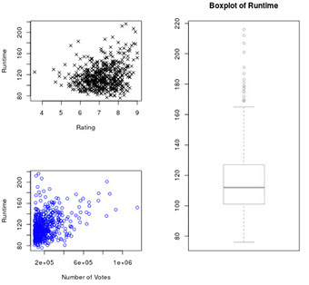
# Build the grid matrix, with 2 scatterplots on the left and a boxplot on the right

grid <- matrix(c(1, 3, 2, 3), nrow = 2, ncol = 2, byrow = TRUE)

 

# Specify the layout

layout(grid)

 

# Build three plots

plot(movies$rating, movies$runtime)

plot(movies$votes, movies$runtime)

boxplot(movies$runtime)

 

# Customize the three plots

plot(movies$rating, movies$runtime, xlab = "Rating", ylab = "Runtime", pch = 4)

plot(movies$votes, movies$runtime, xlab = "Number of Votes", ylab = "Runtime", col = "blue")

boxplot(movies$runtime, border = "darkgray", main = "Boxplot of Runtime")

 

Plot a linear regression

 

# Fit a linear regression: movies_lm

movies_lm <- lm(movies$rating ~ movies$votes)

 

# Build a scatterplot: rating versus votes

plot(movies$votes, movies$rating)

 

# Add straight line to scatterplot

abline(coef(movies_lm), lwd = 2)

 

# Customize scatterplot

plot(movies$votes, movies$rating, main = "Analysis of IMDb data", xlab = "Number of Votes",

ylab = "Rating", col = "darkorange", pch = 15, cex = 0.7)

 

# Customize straight line

abline(coef(movies_lm), lwd = 2, col = "red")

 

# Add text

xco <- 7e5

yco <- 7

text(xco, yco, label = "More votes? Higher rating!")